6.3 Tuning number of topics

https://juliasilge.com/blog/evaluating-stm/

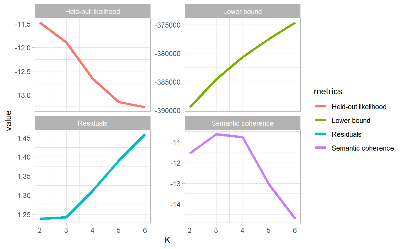
To compare topic models (not necessarily LDA) with different number of topic \(K\), we need first to propose metrics for comparison or topic quality. Semantic coherence s maximized when the most probable words in a given topic frequently co-occur together, which correlates human judgement of topic quality.

https://rdrr.io/cran/stm/man/exclusivity.html

data("data_corpus_inaugural", package = "quanteda")
inaugural_counts <- tidy(data_corpus_inaugural) %>%
  mutate(document = str_c(Year, President, sep = "_")) %>% 
  unnest_tokens(word, text) %>% 
  anti_join(stop_words) %>% 
  count(document, word, sort = TRUE)

inaugural_dfm <- inaugural_counts %>% 
  cast_dfm(document = document, term = word, value = n)

It took several minutes and quite a lot computing power to run the following code. So

library(furrr)
plan(multiprocess)

models <- tibble(K = 2:6) %>%
  mutate(topic_model = future_map(K, ~ stm(inaugural_dfm,
                                           init.type = "Spectral",
                                           K = .,
                                           verbose = FALSE)))

models
#> # A tibble: 5 x 2
#>       K topic_model
#>   <int> <list>     
#> 1     2 <STM>      
#> 2     3 <STM>      
#> 3     4 <STM>      
#> 4     5 <STM>      
#> 5     6 <STM>

heldout <- make.heldout(inaugural_dfm)

k_result <- models %>%
  mutate(exclusivity        = map(topic_model, exclusivity),
         semantic_coherence = map(topic_model, semanticCoherence, inaugural_dfm),
         eval_heldout       = map(topic_model, eval.heldout, heldout$missing),
         residual           = map(topic_model, checkResiduals, inaugural_dfm),
         bound              = map_dbl(topic_model, function(x) max(x$convergence$bound)),
         lfact              = map_dbl(topic_model, function(x) lfactorial(x$settings$dim$K)),
         lbound             = bound + lfact,
         iterations         = map_dbl(topic_model, function(x) length(x$convergence$bound)))

k_result %>%
  transmute(K,
            `Lower bound`         = lbound,
            Residuals             = map_dbl(residual, "dispersion"),
            `Semantic coherence`  = map_dbl(semantic_coherence, mean),
            `Held-out likelihood` = map_dbl(eval_heldout, "expected.heldout")) %>%
  pivot_longer(-K, names_to = "metrics", values_to = "value") %>%
  ggplot(aes(K, value, color = metrics)) +
  geom_line(size = 1.5) +
  facet_wrap(~ metrics, scales = "free_y")